console.blog()

Over the summer, one mini-project that I worked on was implementing a fairly low-level library in C. The original idea was to be able to compile small programs without needing to link against libc. This was reasonably successful (although I haven’t implemented such things as argv), but perhaps the most interesting part of the project ended up being the library of math routines. In this post, I would like to delve into some of the fun things that I learned about approximating functions during these endeavors.

To back up a bit, let’s ask a more fundamental question: what are computers good for? From the name, we can reasonably infer that they compute things. We often take this for granted, but computation is at the heart of what computers do. How, exactly, does the computer compute? Things like addition and multiplication seem relatively simple: after all, I’m capable of adding and multiplying (and by extension, subtracting and dividing) numbers by hand. Surely it’s not too hard to design a circuit to do it?

But what about a more complicated function–take \(\sin x\) or \(\sqrt{x}\), for instance. Except for the trivial values (\(\sin \pi/6 = 1/2\), etc.), there isn’t an obvious way for me to calculate these functions by hand. If I were faced with this question on an exam, I might simply turn to my calculator. But wait a minute–how is my calculator doing it? What sort of algorithms can we use to take the square root or the sine of a number?

The key is to realize that we’re really just approximating the value. For instance, \(\sqrt{2}\) was known by the ancient Greeks to be irrational, so it can’t be expressed in a finite number of decimal places. What the calculator is doing is simply telling me, to some degree of accuracy, that \(\sqrt{2} \approx 1.41421356...\). But how does this happen? What sorts of guarantees can the calculator give me on the accuracy of the approximation? What tradeoffs are there between the speed of an approximation and its accuracy? Hopefully, by the end of this post, you’ll have at least some knowledge of what happens when you make a library call like:

import numpy as np
print np.sin(3.5)

A note on code: throughout this post, I’ll include a few brief Python snippets to enhance the reading experience. If you’re not familiar with Python, don’t worry; the math and theory are still very applicable.

a simple case: the square root function

Let’s start off with one of the most basic functions that we typically turn to a calculator for: \(f : x \mapsto \sqrt{x}\). Approximating the square root of a number is a time-honored tradition; in fact, the ancient Babylonians had a formula for it. The idea behind most approximation algorithms is that we converge to the correct value: we start off with an initial guess and then come up with successively better ones. We’ll call our initial guess \(x_0\) and our \(n\)-th guess \(x_n\). Then the Babylonian formula to compute \(\sqrt{S}\) goes:

The intuition here is remarkably simple: if our guess \(x_n > \sqrt{S}\), then \(S / x_n < \sqrt{S}\); otherwise, if \(x_n < \sqrt{S}\), then \(S / x_n > \sqrt{S}\). Either way, the average of \(x_n\) and \(S / x_n\) can be expected to be closer to the true value of \(\sqrt{S}\), thus giving us an improved guess.

(This is often referred to as Newton’s method because it’s a special case of a more general root-finding algorithm derived by Newton, applied to find the positive root of \(x^2 - S = 0\).) Without going into too much detail, this is an amazing formula: it converges quadratically, meaning that the number of correct digits roughly doubles with each pass. We can test this with a simple Python function:

# use Newton's method to approximate sqrt(S)
# given: original number 'S', initial guess 'x0',
#        and number of guesses to make 'n'
def newton(S, x0, n):
    print x0
    if n == 1:
        return x0
    x = 0.5 * (x0 + S / x0)
    return newton(S, x, n-1)

Using this to approximate \(\sqrt{2}\) with initial guess \(1\) for just four iterations gives (showing the number of correct digits with each pass):

1
1.5  # okay, that's not correct, but I wanted to make a point
1.41
1.41421
1.41421356237

Cool, so now we know how we (and thus a computer) can approximate a relatively “simple” function like the square root. Granted, a real math library like numpy would probably use a slightly more advanced algorithm, but at least we have a clue how we could do it. This gives us the background to move on to a more complex example: the sine function.

a harder case: the sine function

The sine function is really just a glorified wiggly line. It looks¹ something like:

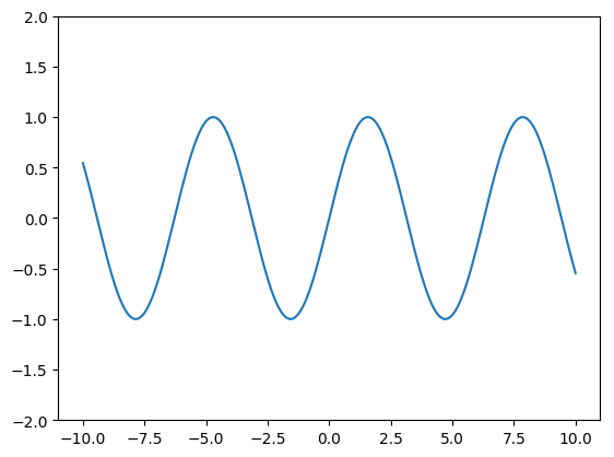
How could we express this function so that we (and thus a computer) could compute an approximation to it? If you’ve taken AP Calculus before, your mind probably just jumped to *shudder* the Taylor series. If you haven’t taken calculus (or have already forgotten it), this basically means that we can use magic to derive the formula:

This, again, is a fantastic approximation. We are rewriting the very complicated sine function as a simple polynomial! The more terms we add, the closer and closer it gets to the real sine function; if we could add infinitely many terms, we would get the true value of \(\sin x\). Even better, there’s a formula that will give us an upper bounds on the error (i.e. guarantee that our guess is within a certain range of the true value), so we know exactly how many terms we need to add if we want our estimate to be within, say 0.000001 of the true value. Is this how computers compute \(\sin x\)?

The answer is a resounding no².

As beautiful as the Taylor series is from an analytical, mathematical standpoint, it’s fundamentally unsuitable for what we’re trying to do here. The issue is that the Taylor series is an approximation of a function about a point. In the above example, we’ve approximated \(\sin x\) in the neighborhood of the point \(x = 0\); it will work beyond this, but we’ll need an increasingly large number of terms. So what do we really want to do? We want to approximate \(\sin x\) across an interval, say the interval \(0 \le x \le \pi/2\). This is a good choice for our interval, since the sine function is periodic: once we’ve approximated it over this interval, we can then repeat it ad infinitum to get the rest of the curve.

But let’s stick with the idea of trying to approximate the function with a polynomial: polynomials are simple and easy to evaluate. It turns out there are many different ways to get a polynomial that resembles the sine curve over this interval, such as the Chebyshev polynomial. However, there really is one that’s “more equal” than the others: the minimax polynomial. It gets its name because it minimizes the maximum error over the interval. Like the Taylor polynomial, it takes the general form:

except with different values for \(a_1, a_3, a_5, ... a_n\); it intuitively makes sense that we would model an odd function like sine with an odd polynomial (and this gives us the interval \(-\pi/2 \le x \le 0\) for free). Calculating the coefficients is much more difficult than it is for the Taylor polynomial (if you’re interested, see the Remez exchange algorithm and the equioscillation theorem). But once we’ve calculated the coefficients once, we can use them over and over again; moreover, the minimax polynomial will generally be orders of magnitude more accurate than a Taylor series of the same degree (in the worst case).

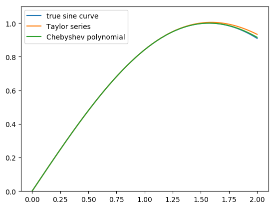
Here’s a a graph of how the real sine function (blue), the fifth-degree Taylor series (orange), and the fifth-degree Chebyshev polynomial (green) compare between 0 and 2:

If you’re still not convinced, here’s a graph showing the absolute error (deviation from the true value of sine) for the same approximations:

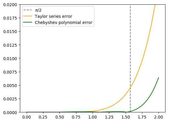
The Taylor series is quite accurate near 0 (the point where the series is centered) and even beats the Chebyshev polynomial in the neighborhood of 0.75; however, the error skyrockets one we get close to π/2, whereas the Chebyshev polynomial keeps a fairly consistent error within our specified interval.

fine-tuning: argument reduction, efficiency

Now we have a good idea of how we (and thus a computer) might take an approximation to \(\sin x\). How can we make our approximation more efficient? After all, time is money. Let’s say we’re writing a math library. How should we implement sine? This seems like a trivial question: we have the polynomial we want; why can’t we just implement it? Let’s look at a naive implementation with a fifth degree Chebyshev polynomial:

# naively compute a fifth-degree polynomial approximation for sine
def sin_cheby(x):
    a1 =  0.999911528379604
    a3 = -0.166020004258947
    a5 =  0.007626662151178
    return a1*x + a3*x*x*x + a5*x*x*x*x*x;

That’s a lot of multiplications (9) and additions (2). If we can somehow reorder the polynomial evaluation to use fewer operations, we can shave off some CPU cycles. Hooray for micro-optimization!

As it turns out, the theoretically most efficient³ way to evaluate a polynomial is use what’s called Horner’s method, which minimizes the number of basic operations needed. In general, a polynomial defined as:

can be most efficiently evaluated as:

Since we have an odd polynomial, we can actually optimize this even further and express it in terms of \(x^2\), leading to the improved version:

# use Horner evaluation to do a faster fifth-degree sine approximation
def sin_cheby(x):
    a1 =  0.999911528379604
    a3 = -0.166020004258947
    a5 =  0.007626662151178
    x2 = x ** 2
    return x * (a1 + x2 * (a3 + x2 * a5))

That’s just 4 multiplications (including evaluating x ** 2) and 2 additions!

But there’s another caveat: our polynomial is only a good approximation of sine from \(-\pi/2 \le x \le \pi/2\). What if the user wants to take the sine of, say, 65? Sine the sine function is periodic, we’re in luck: we just need to somehow transform the angle to get an equivalent angle that’s within our domain. Without getting into the details of floating-point modulus, we can essentially take the angle modulo 2π to get an identical angle inside the unit circle. Then we’ll use the symmetry of the unit circle to get an equivalent angle within our domain. Putting it all together, we get an ultimate sine routine:

# we only import numpy to get an accurate value of pi
from numpy import pi as PI

# an ultimate sine routine for a given angle 'x', in radians
def sin(x):
    # reduce the angle to within -pi/2 and pi/2
    x %= 2*PI
    if x > PI:
      x -= 2*PI
    if x > PI/2:
      x = PI - x
    if x < -PI/2:
      x = -PI - x

    # evaluate the fifth-degree Chebyshev polynomial for sine
    a1 =  0.999911528379604
    a3 = -0.166020004258947
    a5 =  0.007626662151178
    x2 = x ** 2
    return x * (a1 + x2 * (a3 + x2 * a5))

Let’s try it out: with only a fifth degree approximation, we have:

>>> sin(65)
0.8268835613618994

For comparison:

>>> import numpy as np
>>> np.sin(65)
0.82682867949010341

Our little function is just 5.488e-05 off from the true value! That’s a 0.00664 percent relative error. Not bad.

conclusion

Wow, that was significantly longer than I had anticipated. If you’re still here, you hopefully are fairly familiar with what really goes on “behind the scenes” when you try to compute the value of a function like sine on your computer or calculator. Hopefully you also found it at least somewhat interesting; approximation theory is quite interesting because, despite being a branch of mathematics, it’s extremely practical, and you can play with it directly on your computer.

Ms. Agazarian, if you’ve gotten here after grading this post, I’m really sorry for subjecting you to this.

footnotes

¹The graphs in this post were all made using the Python scipy stack. The coefficients of the fifth-degree Chebyshev approximation were computed using sympy.

²Okay, that’s not entirely true. Actually, if you look at, for instance, the glibc implementation of the inverse sine function, you’ll see that they’re actually using the Taylor series. I just wanted to make a point. As a side note, they’re also using the Horner evaluation method discussed in this post.

³Okay, as it turns out, modern CPUs are very complicated, and what’s theoretically optimal for a basic, step-by-step process is not always optimal on actual hardware. As opposed to a simple “do this then do that”, modern CPUs actually work more like “do this and while we’re at it do that and see if it will also simultaneously work on these and those.” Of course, these things have technical names like branch prediction, pipelining, SIMD, etc.

bonus material (further reading)

Real World Example: If you’re feeling adventurous, you can take a look at a real-world implementation of the sine function, using perhaps one of the most widely-used ones: the glibc implementation (for 64-bit doubles, anyway). For those not familiar with C or Linux, glibc is the GNU implementation of the C Standard Library, one of the cornerstones of the POSIX standard. It’s a set of C routines that any conforming operating system must provide, including quite a few math functions. Their sine implementation is a fair bit more complex than the one in this post (they break the input up into several intervals and use different approximations for each one), but it’s sort of cool.

IEEE 754: Throughout all this time, we’ve talked about numbers in computers as if they were practically arbitrary in precision, and basic operations on them (i.e. addition and multiplication) were completely precise. Unfortunately, that’s not the case. The relevant standard for describing how computers implement floating-point numbers is IEEE 754.

Hardware: As it turns out, computing the sine of a value is quite a common task–so common that Intel decided to include an fsin instruction in its x86 architecture. If it’s available on your computer, it seems like this would be the obvious way to go. However, as this blog post shows, sometimes the tried-and-true library functions can be your best bet, and not just for portability reasons.

Another Blog Post: Actually, this post draws inspiration and background material from this post, which is unfortunately not safe for school.