introduction
Continuing my trend of talking about numerical methods for approximating stuff, I’d like to spend this post talking about something I recently heard about and found quite interesting: the possibility of using random simulations to compute integrals. The general idea of the Monte Carlo method (using random simulations to predict non-random but complicated things) apparently first came to John von Neumann and friends while they were working on complicated nuclear math. As always, I think a concrete understanding is extremely valuable, so after presenting the theory, I’ll implement a rudimentary version in Python. It’s not really necessary to have prior Python experience to enjoy this post, but it’d probably be helpful to be familiar with a bit of calculus and statistics. I’ll do my best to review the necessary math as we go along.
Be forewarned that, aside from some classical results, pretty much everything in this post is my speculation and could be very far off from reality.
prelude: random integration?
One of the most important and basic operations in calculus is taking the definite integral of some single-variable function f(x) on some interval between x=a and x=b, denoted:
There are a lot of interpretations of this value, but probably the most straightforward is as the area under the graph of f(x) from a to b; for the concrete example of f(x) = sin(x) from [a,b] = [0,1], this is:
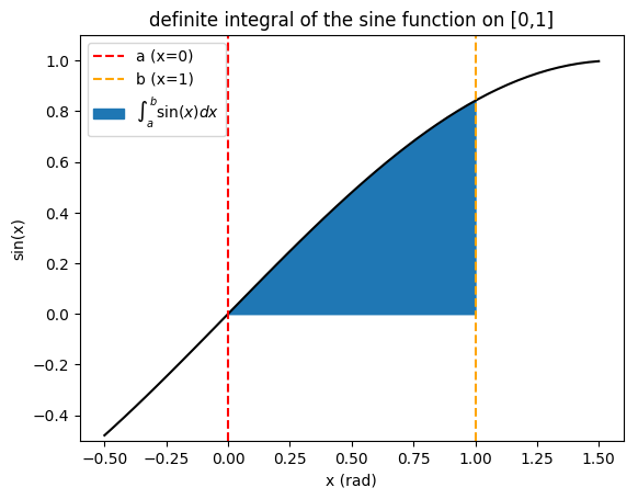
(Source code for this figure is here.)
Definite integrals are very useful, but finding exact, analytic expressions for them can be quite challenging. For the above example, it can be shown that the area is exactly equal to cos(0) - cos(1) = 0.459698..., but for more complication functions, there may be no simple closed-form expression. That’s why very smart people have invented numerical methods for getting extremely good approximations for integrals, such as Simpson’s rule, which breaks the interval into a bunch of parabolic sections that have approximately the area we want.
That’s all well and good, you say, but where does the randomness come into this? I know how to compute Simpson’s rule because it’s on our math midterm; isn’t it an explicit formula? There’s nothing random about it!
And you’re right, we have perfectly good approximations for single-variable integrals that don’t involve randomness. But what if you have a really nasty triple integral or something? Then you wouldn’t want to follow a rigid formula. Instead, we guess! (Well, educated mathematical guessing, that is.) So just how do we go about randomly guessing integrals in a scientific manner?
the mean value theorem
A famous result from AP Calculus BC is the mean value theorem for integrals, which states that the average value of a function on an interval can be found in terms of its definite integral over that interval. More specifically:
\[\bar{f}(x) = \frac{1}{b - a} \int _a ^b f(x)\,dx\]Usually, we know the definite integral and use it to figure out the average value of the function. But, being the clever and mathematically rebellious souls that we are, why don’t we try the opposite problem: finding the average value first and then using it to approximate the integral? Aha!
Now how can we find the average value of the function? For some functions, it’s trivial; for example, if it’s a linear function, just take the midpoint of the line. But for a function like sine, it’s not exactly obvious.
This is where the randomness comes in: instead of scratching our heads trying to figure out how to get a good approximation of the average value, why don’t we randomly generate a bunch of \(x\) in the interval and then find the average value of the \(f(x)\) values? With the help of numpy’s random number generator, we can implement this in Python:
import numpy as np

# use mean value theorem to estimate integral of f on [a, b] using n samples
def mc_int(f, a=0, b=1, n=5000):
    xs = np.random.random(n) * (b - a) + a
    ys = map(f, xs)
    return np.average(ys) * (b - a)
Let’s test it:
>>> mc_int(np.sin)  # sine function on default interval of [0,1], 5000 trials
0.45563403636694083
# pretty close to the Wolfram Alpha answer of 0.4596976941318602825990634
This is a decent estimate. One major drawback is that it’s rather slow: generating lots of random numbers is hard for a computer, which is a pretty deterministic machine. (Actually, these numbers are really pseudo-random, but that’s a topic for another blog post.)
can we quantify the random?
One issue with this method, besides the fact that it’s inefficient, is that it always relies on some degree of randomness: unlike, say, the hard bounds on the precision of a series approximation or Simpson’s method, we can never be exactly sure of our results. However, based on the randomness inherent in our simulation, we can still describe what we’d expect to see. Fortunately, there’s an entire branch of math dedicated to figuring out how lots of random behavior works out in the long run…statistics!
One of the greatest classical results of statistics is the central limit theorem, which states that, irrespective of the distribution of a random variable, if you take a large sample of that variable and find the average, the sampling distribution of the averages is our good friend the normal distribution! I don’t know the proof, but this extremely surprising and important result is due to the French mathematician Laplace; it’s said that his contemporaries did not quite realize its central importance in the field of statistics. I’ll let Wolfram Alpha describe this more precisely:
Then the normal form variate…has a limiting cumulative distribution function which approaches a normal distribution
the variate…is normally distributed with μX=μx and σX = σx/√n
So we’d expect our simulated integral values (which are themselves the results of thousands of simulations) to be normally distributed with a mean μ at the true value of the integral. We don’t know the exact standard deviation σ of the population, but we can make an educated guess in each trial by dividing the standard deviation of the trial y-values by the square root of the sample size.
This all leads to the next point: by using the Monte Carlo method of simulation, we’ve obtained an educated (random) guess of the true value of the integral. But how far off should we expect to be? How confident are we in our guess?
If you haven’t guessed already, we’ll set up a confidence interval to find out. Statistically speaking, based on our simulation, we want to come up with a range of values (called the confidence interval) where we’d expect the true value to lie. The size of this range (called the margin of error) depends on how confident we want to be in the result. Let’s say I run the simulation for sin(x) on [0,1] and I get 0.45 as my approximate value. I could claim that the true value of the integral is exactly 0.45 (equivalent to asserting a margin of error of 0)…if I’m willing to be 0% confident in my result. On the flip side, I could be 100% confident in my result…if I claim an infinitely large margin of error. Neither of these things is particularly useful.
If I want to assert a more useful margin of error, I’ll have to quantify how likely it is for my confidence interval to capture the true value. Recall that, for the standard normal distribution, the z-score tells us how many standard deviations away from the mean any given data point lies. Now let’s say I arbitrarily want to find an interval in which I can have 95% confidence that I’m right. Essentially, I want to find some critical z-score (we’ll call it z*) that makes the probability of finding the mean between -z* and +z* standard deviations away 0.95. We can find such a z* by inverting the normal cumulative distribution function, which I’ll do here using norm.ppf (“normal percent point function”) from the scipy package:
from scipy.stats import norm

print norm.ppf(0.975)  # central area of 0.95 + one tail area of 0.025
I get something like 1.95996398454 standard deviations. So, 95% of the time, I’d expect the true mean to fall within z* = 1.96 standard deviations away from my guess. We can pretty easily compute the size of the standard deviation of the random sample; because I’m lazy, I’ll cheat and use np.std(ys, ddof=1), where we set the degrees of freedom to 1 because this is a sample. The central limit theorem tells us that we should expect the population standard deviation to be this divided by the square root of the sample size, which in this case happens to be n = 5000. How far away we’ll be 95% of the time is then simply z*, the number of standard deviations, times the size of one standard deviation, which we compute for each trial.
One last caveat: we often describe levels of confidence in terms of an α-value, which is just 1 minus the level of confidence. So for 95% confidence, we have α = 0.05. Now we’re ready to implement this in Python, building on our program from earlier:
def mc_int(f, a=0, b=1, n=5000, alpha=0.05):
    xs = np.random.random(n) * (b - a) + a
    ys = map(f, xs)
    res = np.average(ys) * (b - a)

    # get critical z-score and margin of error
    z = norm.ppf(1.0 - alpha / 2.0)
    margin = z * np.std(ys, ddof=1) / np.sqrt(n)

    # we expect the true value of the integral to be within
    # res - margin and res + margin about 95% of the time
    # we'll return our guess res along with this confidence interval
    return res, res - margin, res + margin
Let’s test it:
>>> mc_int(np.sin)
(0.4638704415461013, 0.45708884281589718, 0.47065204027630542)
# and...the true value is indeed within the interval!
repetition makes perfection
So we’ve worked out the theory for the confidence intervals on this integral, but does it actually work? Since this is all my own speculation, I have no idea, but we can do a simulation to test if it seems to be working. Recall that an alpha value of 0.05 (95% confidence) means that we expect that, if we repeatedly generate confidence intervals, 95% of them will capture the true value. Why don’t we set up a simulation to test our simulation? (That’s pretty meta.) We’ll set up the simulation parameters:
N = 5000  # number of trials
true_val = 1 - np.cos(1)  # the true value of the integral
Then, we’ll call mc_int a total of N times and count what percentage of the confidence intervals successfully captured the true value:
print np.average([2 * np.abs(res - true_val) < hi - lo
                  for res, lo, hi in [mc_int(np.sin) for _ in range(N)]])
(Here, I take advantage of the Python convention that True == 1 to abbreviate the code. Also, the 2 is because the interval is symmetric: the margin extends on both sides.) It takes a bit to run, but we end up with 0.9474, which is almost exactly the 95% that we’re supposed to be getting. Until someone comes up with a more advanced mathematical analysis that proves me wrong, I’ll assume that our function works perfectly!
conclusion
Well, this was a pretty fun journey. We got to see how, through the careful application of statistics, we can use random simulations to approximate complex deterministic phenomena, using the example of a definite integral. Maybe someone can come up with a better simulation for doing this than the basic average value one I used.
(The code in this post was sort of all over the place; while I think it flowed better with the exposition, it’s probably difficult to gather in one place. If you’d like a copy, I’ve complied the important bits here.) (Does that make me a literate programmer?)
corrigendum
I didn’t want to edit the post body (because the deadline for the marking period 2 assignment has already passed), but I noticed that the logic in that last code example is pretty convoluted. I think a much clearer version is:
print np.average([lo <= true_val <= hi
                  for _, lo, hi in [mc_int(np.sin) for _ in range(N)]])
A second (slight) adjustment: after learning some more in Mrs. Brown’s statistics class, it seems like it would be more suitable to use a t-distribution for this post, since we lose an independent degree of freedom when we estimate the population variance with that of our random sample. However, the result should be quite similar, so I won’t bother re-writing the entire post except to leave this note here. I suppose it just goes to show that there’s always a way something can be improved, although it sometimes takes hindsight to realize it.