console.blog()

introduction

In stat class, one of our favorite calculator functions is the good old normcdf, which finds the probability that, when we sample a random variable, we’ll get something within a certain range. As implemented on the trusty TI-nspire, it can seem like black magic: you put some numbers in, and out pops your perfect AP Stat score! I wanted to write a post demystifying this process a bit. First, we’ll clarify what we mean by the normcdf function. Then, we’ll take a look at the mathematical building blocks for the function. Finally, we’ll implement it in Python.

This post should be accessible to anyone who is currently taking AP Stat, has a cursory familiarity with Python, and has an AP Calc BC-level understanding of series. Even without the Python, the math part is (hopefully) interesting.

prelude: what’s normal, anyway?

We generally have a vague notion that a “normal” distribution is a probability distribution that’s bell-shaped. For example, take the heights of students in a school: when we say that this variable (height) is normally distributed, we mean that the frequencies sort of look like this:

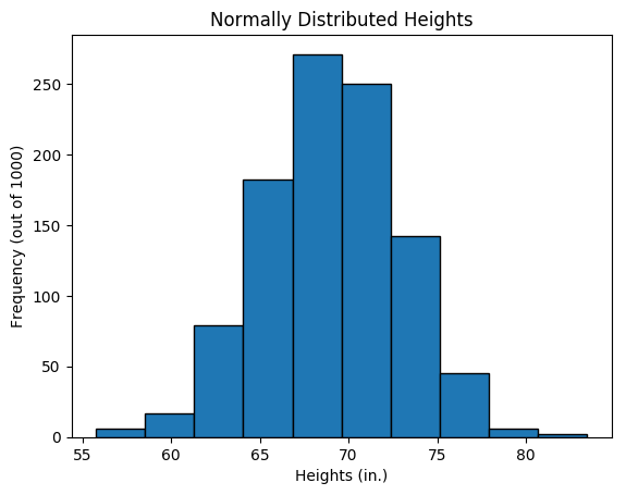
The above distribution is what we call discrete, since there are finitely many data points. Now imagine that we have an infinitely large population: the distribution would get smoother and smoother until we have a continuous curve like the one below:

Here, the y-axis is the relative frequency of a given x-value’s occurrence. Let’s get slightly more technical with how we describe this distribution. When we talk about a normal distribution, there are really two parameters that we need to take care of: \(\mu\) (the mean, or the height we would expect from an average person) and \(\sigma\) (the standard deviation, or roughly how far we would expect any given person to fall away from our mean). You can also think of \(\sigma\) as how spread out the height values are. To make this clearer, here’s the same continuous distribution with the mean height and a height one standard deviation above the mean labeled:

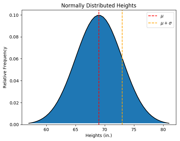
For this simulation, I arbitrarily set \(\mu = 69\) and \(\sigma = 4\).The key takeaway is that with a continuous distribution, we’re not really interested in the relative frequency of a given height (let’s just say the mean height \(\mu\) as an example). Since there are infinitely many possible heights, the probability of any given height being exactly 69 is zero! What is meaningful is the total probability within a given interval—in the plot above, let’s say the probability between the mean \(\mu\) and one standard deviation above the mean, or \(\mu + \sigma\). Since the curve is normalized (i.e. the total blue area is equal to 1), the probability of any randomly selected height \(x\) falling within \(\mu \le x \le \mu + \sigma\) is simply the cumulative area between the red and orange lines. To give a concrete example, for the above distribution, the probability of randomly selecting a height \(x\) such that \(69 \le x \le 73\) is the cumulative distribution function¹ under this normal curve. In other words, the normcdf from 69 to 73.

(note: the code I used to generate these graphs can be found here)

mathy stuff

Now, if you’ve taken AP Stat, I probably haven’t told you anything new yet. I just wanted to provide a quick refresher on the normal distribution; here’s where the new stuff comes in. As you probably guessed when I mentioned the area under the curve, the normcdf function is really just the integral of the probability function (shown as the black curve in the graph above and referred to as a normpdf on the calculator). So, if we know the equation for the black curve, we should be able to integrate it and get an expression for normcdf, right?

Well, reality is unfortunately slightly more complicated than that. You may have heard the normal distribution referred to as the “Gaussian” distribution². That’s because the pdf function for generating it (technically called the “kernel function”) is the Gaussian function, or:

where \(\mu\) and \(\sigma\) are our friends mean and standard deviation from before. Really, we just want the area under the curve from \(a\) to \(b\):

That doesn’t look too troublesome to integrate, but if you try, you’re guaranteed to fail: there isn’t any elementary antiderivative. This means that there is no combination of “basic” functions like sine, log, etc. whose derivative is our buddy \(p(x)\). Whelp. We’re going to have to use numerical methods to approximate it.³

implementing erf(x)

Let’s use the time-honored method of getting unstuck and take a step back to look at a “completely different” function, which we’ll call the error function, or erf. (Quite an unfortunate name, really…) This function is defined as:

Well, this is slightly better, but we’re still no closer to actually getting the antiderivative. Gee, if only the integrand were something easy, like a polynomial. We can do polynomials all day long…

Huh. What if we used the Taylor series of \(e^x\) to re-express the integrand as a polynomial? Then we could easily get an infinite series that converges to the value we want, erf(x)! Recall from AP Calc BC that the series expansion for \(e^x\) is:

So that pesky little integrand is really just:

That doesn’t look so intimidating any more. Let’s just integrate it to get:

Or, with the ever-so-elegant summation notation:

Now, this is really an approximation of the true value of erf(x); we’d have to sum an infinite number of terms to get the real value. That’s not very useful, but the good thing is that we can get arbitrarily close to the true value of erf(x) by adding just a finite number of terms. Because this is an alternating series, the maximum possible error of the approximation up to \(n\) terms is simply bounded by the absolute value of the nth term, a famous result from AP Calc BC.

To recap this section, I can’t really find a “closed-form” expression for erf(x), but I can get arbitrarily close to it by adding up the terms of the series shown above. Once the terms I’m adding get below my desired precision \(\epsilon\), I’m guaranteed to have the value of erf(x) to within \(\epsilon\).

(Yes, we could have jumped directly to the Taylor series for normcdf, but it isn’t as insightful, and the erf function is important in its own right.)

putting the math together

Okay, so we have a great approximation for erf(x), a function very close to the Gaussian integral that we were trying to approximate in the first place. How do we proceed from here?

Well, let’s revisit another friend from AP Statistics, the z-score. The z-score tells us how many standard deviations a given x-value is from the mean and is defined by:

Note that this looks suspiciously like the exponent in the Gaussian function: it’s really just a scaling factor for the normal distribution. All normal curves are equal, but there’s one that’s more equal than the rest: the standard normal curve, which is just a normal distribution with \(\mu = 0\) and \(\sigma = 1\). We really like this one because the numbers are pretty easy to work with (if you’re in Mrs. Brown’s AP Stat class, the standard normal distribution is what’s on the infamous green sheet).

It turns out that any normal distribution is really just the standard normal distribution, scaled up by a factor of \(z\). Taking advantage of the \(z\) substitution and that \(\sigma^2 = 1\) for the standard normal, let’s simplify our normcdf(a,b) function to look like:

Now, we’ll just use some basic integral rules and the substitution \(u = z/\sqrt{2}\) to get:

Aha! We can now see that:

putting the code together

Honestly, I could probably stop here, but this is supposed to be a coding blog, so I might as well write some code. (Also, I have a lovely Markdown code highlighting thing here, and it’d be a shame not to use it.) Let’s implement our original erf(x) function in Python:

# computes error function to desired accuracy epsilon
def erf(x, epsilon=0.000001):
    # since erf(x) is symmetric, we only focus on x > 0
    y = abs(x)

    # adjust epsilon to account for normalization at the end
    k = 1.1283791670955125739  # this is 2/sqrt(pi)
    epsilon /= k

    # compute the Taylor series about zero
    # use the alternating error term to know when to stop
    term = y
    n = 0.0
    sign = +1.0
    factorial = 1.0
    power = y
    result = term
    while term > epsilon:
        n += 1
        factorial *= n
        sign = -sign
        power *= y * y
        term = power / (factorial * (2 * n + 1))
        result += sign * term

    # normalize and return result
    if x < 0:
        return -k * result
    return k * result

Let’s test it:

>>> erf(0.13)
0.14586711478
# according to Wolfram Alpha, the result should be 0.145867

And now for the finishing touches:

# computes normal cumulative distribution function from lower bounds a,
# upper bounds b, mean avg, standard deviation stdev, and desired accuracy
# epsilon
def normcdf(a, b, avg=0.0, stdev=1.0, epsilon=0.000001):
    # get z scores
    z_a = (a - avg) / stdev
    z_b = (b - avg) / stdev
    k = 0.7071067811865475244008  # this is 1/sqrt(2)

    # because we multiply by 0.5, we shouldn't need to scale epsilon
    return 0.5 * (erf(k * z_b, epsilon) - erf(k * z_a, epsilon))

With fingers crossed, let’s try it:

>>> normcdf(-0.3, 0.1, 0.8, 0.5)
0.0668532280857
# according to the calculator, the result should be 0.06685331227
# perfectly within our 0.000001 precision

Yay, it works! (If you don’t want to copy/paste, you can grab a copy of the code from the comfort of your own home here.)

conclusion

Math, and especially statistics, can seem like a black box at times. But with the power of Python, you can peer into the black box!

If you’re interested in this sort of stuff, here’s some food for thought: the Taylor series we used to approximate erf(x) was centered around 0, which means it really works best for small values of x. It would still give us the right answer for really large x, but it would be terribly inefficient. Can you come up with a better approximation for larger numbers?

footnotes

¹Sometimes, normcdf is called the normal cumulative density function, but for the purposes of this post, the distinction between a probability density function and probability mass function isn’t important. I’ll just call it the distribution function.

²What is it with this Gauss guy? Wikipedia has an entire page devoted to things named after him!

³Interestingly, even though the indefinite integral of \(p(x)\) has no elementary form, the definite integral from negative infinity to infinity can be found using polar trickery. It turns out to be the reciprocal of that coefficient in front, which really just exists to normalize the function.