console.blog()

You’ve probably heard of quantum computing: exploiting quantum phenomena (superposition, entanglement, etc.) to do things that classical computers cannot. You’ve probably also heard of the cloud: a nebulous network of computers that enables magic services like Google Drive. But have you heard of cloud quantum computing?

No, cloud quantum computing is not just a mash-up of several hot buzzwords; look, there are even legit papers about it! It must be a real thing!

Normally, a quantum compter is not the sort of tech an average citizen might have access to. But this is something really cool I just found out about the other today: through the IBM Quantum Experience, you can write code and have it executed on an actual quantum computer! For free! Essentially, IBM has decided to hook some of its prototype quantum computers up to the cloud for random people on the Internet to mess around with. (They aren’t the first or only company to do this, but they’re the only one I’m familiar with using.) Granted, it’s a 5-bit machine, but it’s still very cool. I’d like to spend this blog post walking you though writing a very simple program and executing it on the IBM Yorktown device.

the quantum code

I won’t go into the exact physics¹, but the program I’d like to run (in qasm, quantum assembly) is:

include "qelib1.inc";
qreg q[2];  // two-bit quantum register for computation
creg c[2];  // two-bit classical register for results

h q[0];  // apply a Hadamard gate to the first qubit
h q[1];  // apply two Hadamard gates to the second qubit
h q[1];

measure q -> c;  // measure the results

(Actually, IBM has an open-source Python API, but I think this post is complicated enough without bringing extra libraries in.)

At this level, quantum “programs” are really more akin to constructing circuits than writing software. Much like in classical digital electronics, we start off with some qubits and then apply some gates to perform calculations on them. The program shown above represents the quantum circuit:

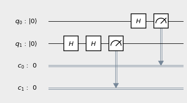
To summarize a fair bit of physics, here’s what the circuit is actually doing:

1. The first qubit (\(q_0\)) starts off in the \(\vert 0 \rangle\) state—this is the quantum equivalent of a \(0\) bit.
2. A Hadamard logic gate (\(H\)) is applied to it. This essentially acts as a randomizer, turning the qubit from a definite \(\vert 0 \rangle\) state to a superposition of the \(\vert 0 \rangle\) and \(\vert 1 \rangle\) states.
3. \(q_0\) is measured, with the result stored in the first classical register bit (\(c_0\)). After the randomization, we would expect a 50% probability of measuring in the \(\vert 0 \rangle\) state and a 50% probability of measuring in the \(\vert 1 \rangle\) state.
4. Likewise, the second qubit (\(q_1\)) is prepared in the \(\vert 0 \rangle\) state.
5. \(q_1\) is “randomized” twice. If this were a classical system, we would expect \(q_1\) to be in a similar superposition of \(\vert 0 \rangle\) and \(\vert 1 \rangle\). Spoiler: quantum mechanics would beg to differ.
6. \(q_1\) is measured, with the result stored in the classical bit \(c_1\). Again, we’d classically expect a 50/50 split between measuring a \(0\) and a \(1\).

the fun part: running the code

Let’s type this code into the qasm editor in the IBM website and send off a request to the Yorktown queue. Whenever the IBM quantum computer is ready, our code will be loaded and run 1024 times, and the results will be emailed to us.

Well, when I ran it (well, technically from cached results to save credits, but that’s a technicality), here’s what I got:

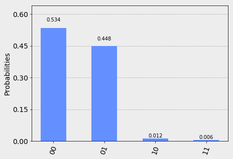
How should we interpret this lovely graph? For each run of the program, our results are contained in the classical register bits \(c_0\) and \(c_1\). Since these are classical bits, they each have two possible states: \(0\) and \(1\). Thus, there are four possible outcomes for each program run: \(00\), \(01\), \(10\), and \(11\), where the right-most bit represents \(c_0\). For example, the \(01\) result tells us that \(q_0\) measured \(1\) and \(q_1\) measured \(0\). The graph is telling us the frequency distribution of results over 1024 runs.

hold on…what just happened?

We said that, from a classical standpoint, we’d expect both \(q_0\) and \(q_1\) to be completely random: that is, the distribution should be roughly uniform. The graph we got is nowhere near uniform. Let’s break down what happened.

The \(q_0\) qubit behaved exactly as we (classically) predicted: it was \(0\) half the time and \(1\) half the time. On the other hand, what’s going on with the \(q_1\) qubit? Though there is some noise because real quantum computers are imperfect, it seems to be biased toward the \(0\) state!

The reason this occurs is the weirdness of quantum mechanics. Just like light waves can interfere with each other and cancel out in classical physics, probabilities can interfere and cancel in quantum. Very roughly speaking, applying the Hadamard gate twice canceled out the randomizations², leaving us in the state we were originally in (i.e. \(0\)). How very strange.

bonus: entanglement at a glance

You might be thinking: this is all well and cool, but what can you really do with five qubits? You’d be right: could quantum computing is currently more of a novelty than anything else. (Although some researchers have done serious computations this way; I think I linked one such paper in the introduction, and I know others have successfully performed Bell violations³.) But there are some surprisingly practical things you can do with the IBM computer, such demonstrating what’s perhaps the most famous quantum effect of them all: entanglement. This is the effect that Dr. Einstein famously described as “spooky action at a distance.”

The actual math is complicated (and honestly, it doesn’t make sense even if you know the math), so I’ll just present the circuit without explanation:

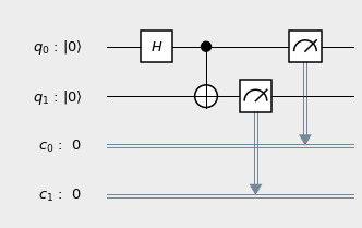
This will cause \(q_0\) and \(q_1\) to become entangled. When we measure them, their values should be completely random but exactly the same. Let’s run it:

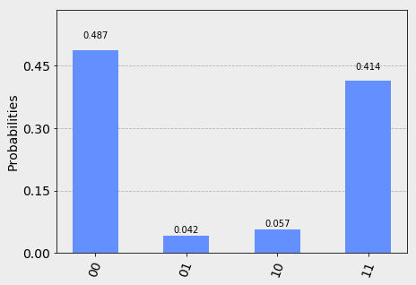
With a little bit of noise due to physical imperfections in the IBM superconducting qubits, this is exactly what we’d expect: a 50/50 distribution of \(00\) and \(11\).

(I generated the figures in this post in Python with the qiskit package. Unfortunately, the code is not available like usual, since I made them in a Jupyter notebook and didn’t save some of it.)

footnotes

¹If you’d like to learn more about quantum computing, I can recommend Professor Mermin’s book on the subject. If you’d like to learn more about quantum in general, check out the second volume in Professor Susskind’s The Theoretical Minimum series.

²Okay, here’s a more formal explanation: gates are unitary linear operators acting on a state space of qubits. In the matrix formulation of quantum mechanics, the Hadamard gate (in the computational basis) is given by:

If we apply \(H\) once, we randomize a qubit. However, if we apply it twice, we get back the original qubit, since \(H^2 = I\), the identity matrix. Try the matrix multiplication yourself!

³The Bell inequalities are a class of experimentally testable statements that statistically show that the world obeys the strange laws of quantum mechanics and not the nice rules of classical mechanics. Bell showed that, unless the world is super-deterministic, the principles of locality and objective reality (i.e. a hidden variable theory) cannot both hold. Actually, since Bell proposed his famous theorem, we’ve come up with even better evidence for quantum mechanics in the form of GHZ tests.